Correspondence Problem
Feature Correspondence
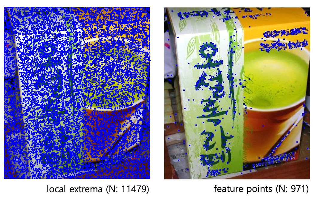
Overview of Feature Correspondence
Features- Corners: Harris corner, GFTT (Shi-Tomasi corner), SIFT, SURF, FAST, LIFT, …
- Edges, line segments, regions, …
Feature Descriptors and Matching- Patch: Raw intensity
- Measures: SSD (sum of squared difference), ZNCC (zero normalized cross correlation), …
- Floating-point descriptors: SIFT, SURF, (DAISY), LIFT, …
(e.g. A 128-dim. vector (a histogram of gradients))
- Measures: Euclidean distance, cosine distance, (the ratio of first and second bests)
- Matching: Brute-force matching ($O(N^2)$), ANN (approximated nearest neighborhood) search ($O(\log{N})$)
- Pros (+): High discrimination power
- Cons (–): Heavy computation
- Binary descriptors: BRIEF, ORB, (BRISK), (FREAK), …
(e.g. A 128-bit string (a series of intensity comparison))
- Measures: Hamming distance
- Matching: Brute-force matching ($O(N^2)$)
- Pros (+): Less storage and faster extraction/matching
- Cons (–): Less performance
- Patch: Raw intensity
Feature Tracking(a.k.a. Optical Flow)- Optical flow: (Horn-Schunck method), Lukas-Kanade method
- Measures: SSD (sum of squared difference)
- Tracking: Finding displacement of a similar patch
- Pros (+): No descriptor and matching (faster and compact)
- Cons (–): Not working in wide baseline
- Optical flow: (Horn-Schunck method), Lukas-Kanade method
Features
Harris Corner (1988)
-
Key idea: Sliding window
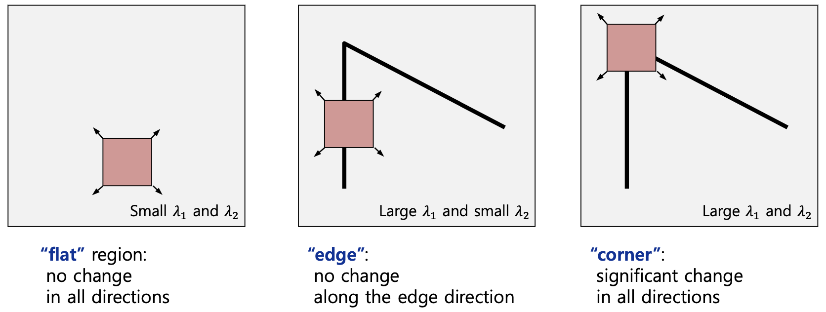
-
Properties
- 불변성
- tranaltion
- rotation
- intensity shift ($I$→$I+b$)
- 가변성
-
image scaling
-
- 불변성
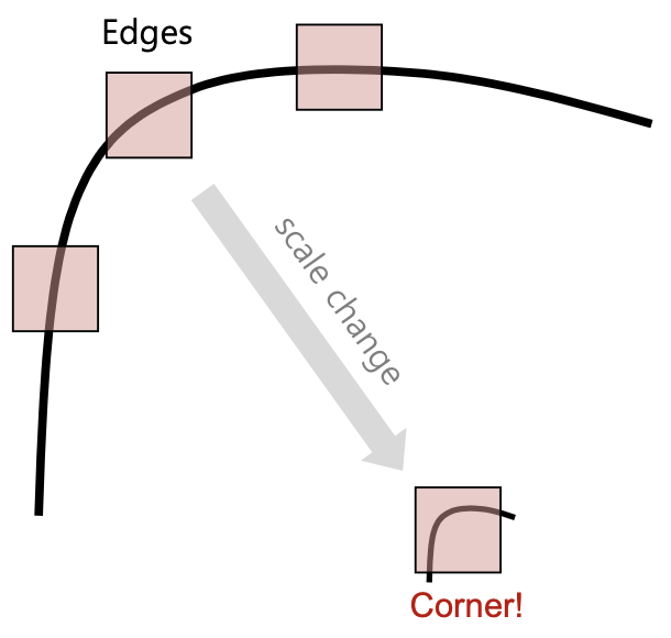
SIFT (Scale-Invariant Feature Transform; 1999)
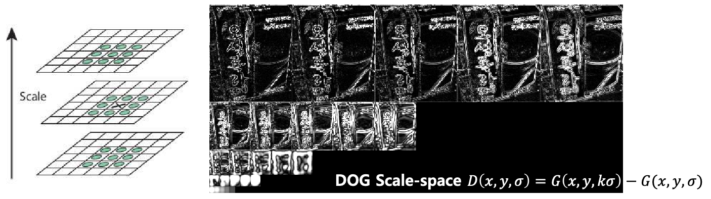
- Key idea: Scale-space (~ image pyramid)
- Part #1) Feature point detection
-
DOG scale-space에서 local extrema (minima and maxima) 찾기
- sub-pixel level에서 3D quadratic function를 사용해 위치를 정확하게 로컬화
-
낮은 대비(low contrast)를 갖는 후보군 제거, $ D(\mathbf{x}) <\tau$ - edges위에 있는 후보군 제거, $\frac{\operatorname{trace}(H)^2}{\operatorname{det}(H)}<\frac{(r+1)^2}{r} \text { where } H=\left[\begin{array}{ll}D_{x x} & D_{x y} \D_{x y} & D_{y y}\end{array}\right]$
-
FAST (Features from Accelerated Segment Test; 2006)
-
Key idea: $N$개 또는 그 이상 픽셀들의 연속적인 호(arc)
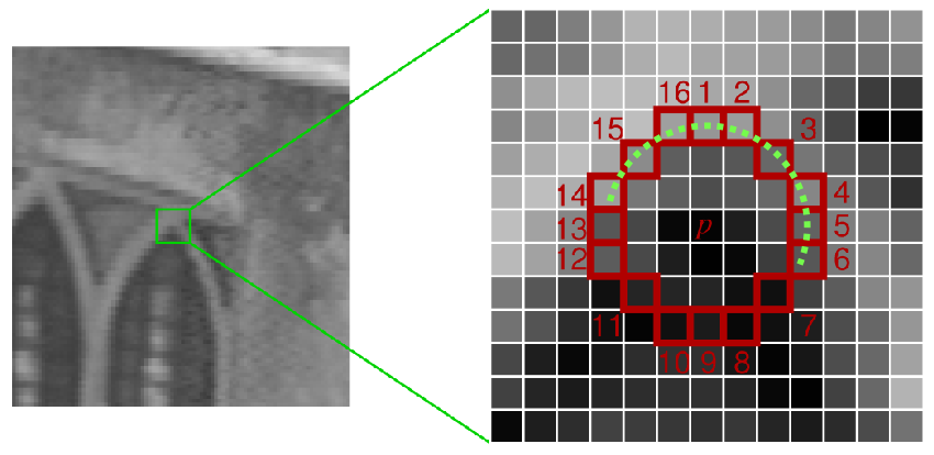
- 이번 patch는 corner인가?
- segment가 $p+t$보다 밝은가?
- segment가 $p-t$보다 어두운가?
- $t$: 유사한 intensity 판별의 threshold
- corner가 너무 많기 때문에 NMS(Non-Maximum Suppression) 필요
- NMS: high confidence를 갖는 것만 남기고 나머지는 제거
- 이번 patch는 corner인가?
-
Versions
- FAST-9 ($N$: 9), FAST-12 ($N$: 12), …
- FAST-ER
- 더 많은 픽셀로 반복성을 향상 시키기 위해 decision tree를 training
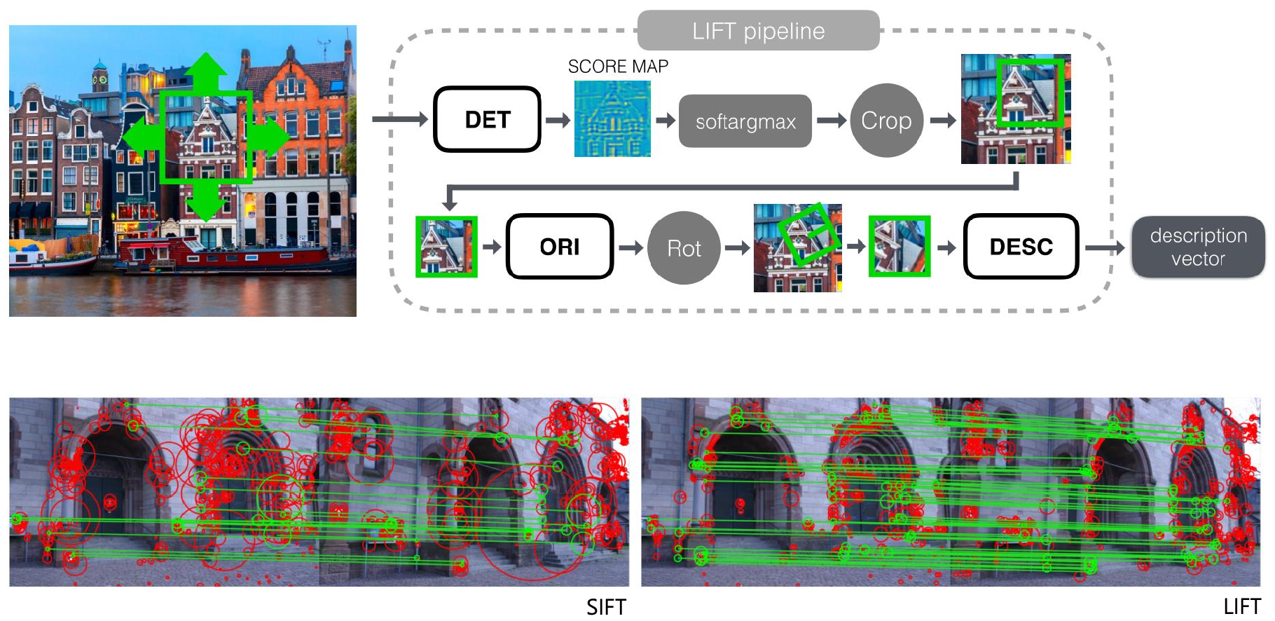
LIFT (Learned Invariant Feature Transform; 2016)
- Key idea: Deep neural network
- DET (feature detector) + ORI (orientation estimator) + DESC (feature descriptor)
Feature Descriptors and Matching
SIFT (Scale-Invariant Feature Transform; 1999)
-
Part #2) Orientation assignment
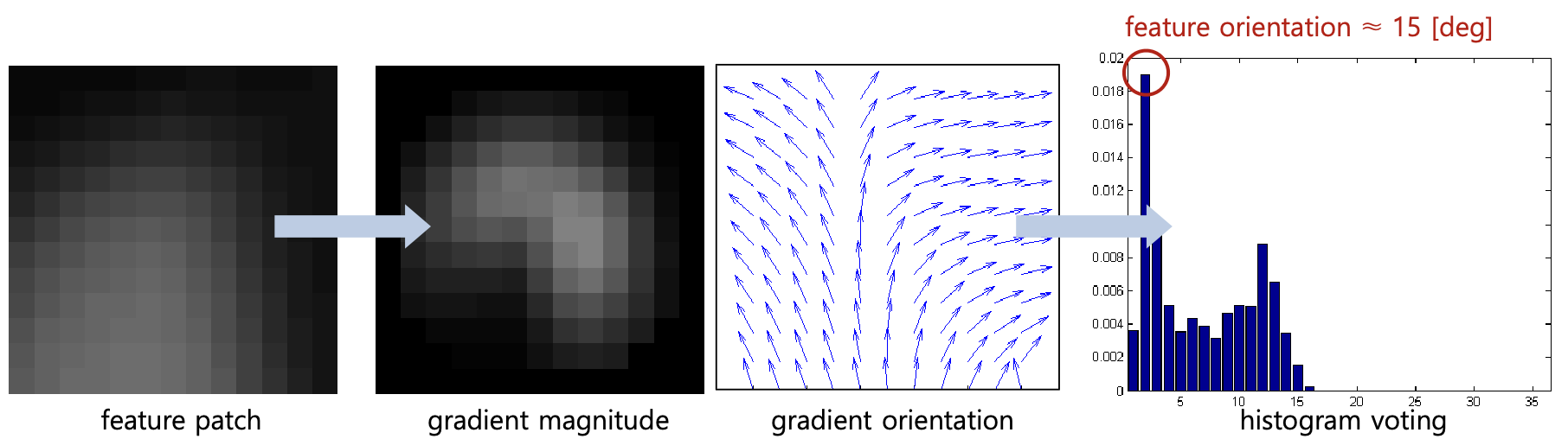
-
각 patch gradient의 magnitude와 orientation 유도
$\begin{aligned}&m(x, y)=\sqrt{(L(x+1, y)-L(x-1, y))^2+(L(x, y+1)-L(x, y-1))^2} \&\theta(x, y)=\tan ^{-1} \frac{L(x, y+1)-L(x, y-1)}{L(x+1, y)-L(x-1, y)}\end{aligned}$
-
가장 강한 orientation 찾기
→ Histogram voting (36 bins) with Gaussian-weighted magnitude
-
-
Part #3) Feature descriptor extraction
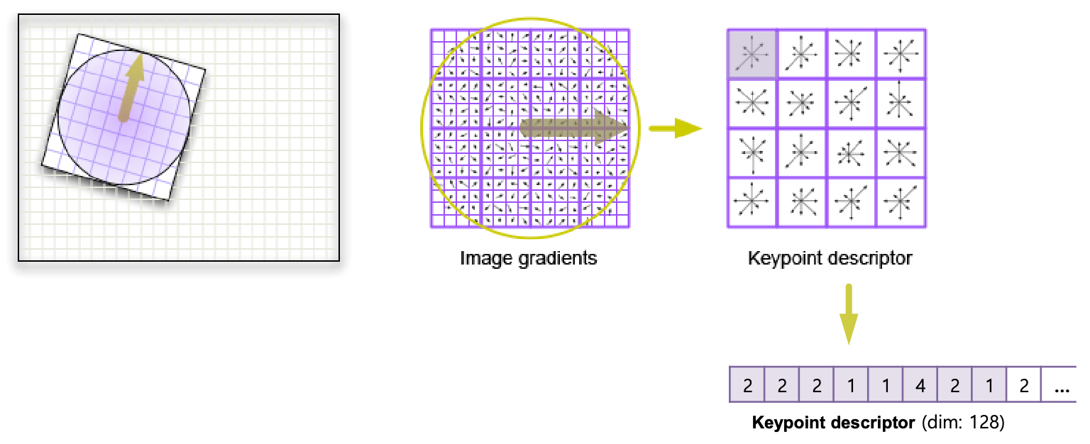
- 각 patch (16x16 pixels)에서 4x4 gradient histogram (8 bins) 사용
- Gaussian-weighted magnitude를 다시 사용
- 할당된 feature orientation에 대한 상대 각도 사용
- histogram을 128 차원 벡터로 인코딩
- 각 patch (16x16 pixels)에서 4x4 gradient histogram (8 bins) 사용
BRIEF (Binary Robust Independent Elementary Features; 2010)
- Key idea: 랜덤한 쌍의 sequence of intensity 비교
- stability와 repeatability을 위한 smoothing 적용
- Path size: 31 x 31 pixels
- Versions: The number of tests
- BRIEF-32, BRIEF-64, BRIEF-128, BRIEF-256 …
- Examples of combinations
- CenSurE detector (a.k.a. Star detector) + BRIEF descriptor
- SURF detector + BRIEF descriptor
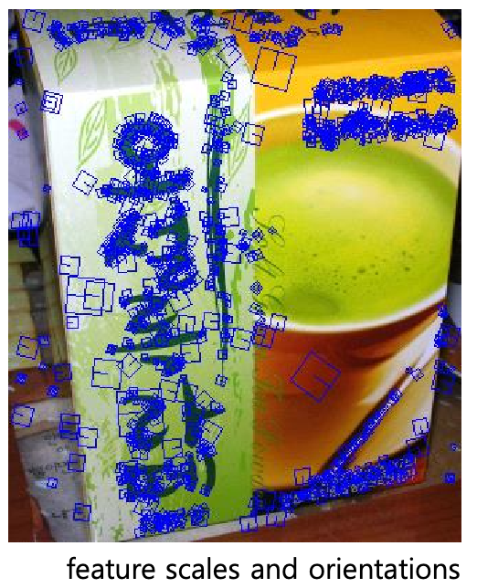
ORB (Oriented FAST and rotated BRIEF, 2011)
- Key idea: BRIEF에 회전 불변성(rotation invariance) 추가
- Oriented FAST
- scale invariance을 위한 scale pyramid 생성
- FAST-9 points 검출 (filtering with Harris corner response)
- intensity centroid에 의한 feature orientation 계산 ⇒ $\theta=\tan ^{-1} \frac{m_{01}}{m_{10}} \quad \text { where } \quad m_{p q}=\sum_{x, y} x^p y^q I(x, y)$
- Rotation-aware BRIEF
- known orientation에 대한 BRIEF descriptors 추출
-
greedy search에 의해 train된 비교 쌍들을 사용
- Oriented FAST
- Combination: ORB
- FAST-9 detector (with orientation) + BRIEF-256 descriptor (with trained pairs)
- Computing time (@ 24 images (640x480) in Pascal dataset)
- ORB: 15.3 [msec] / SURF: 217.3 [msec] / SIFT: 5228.7 [msec]
Feature Tracking
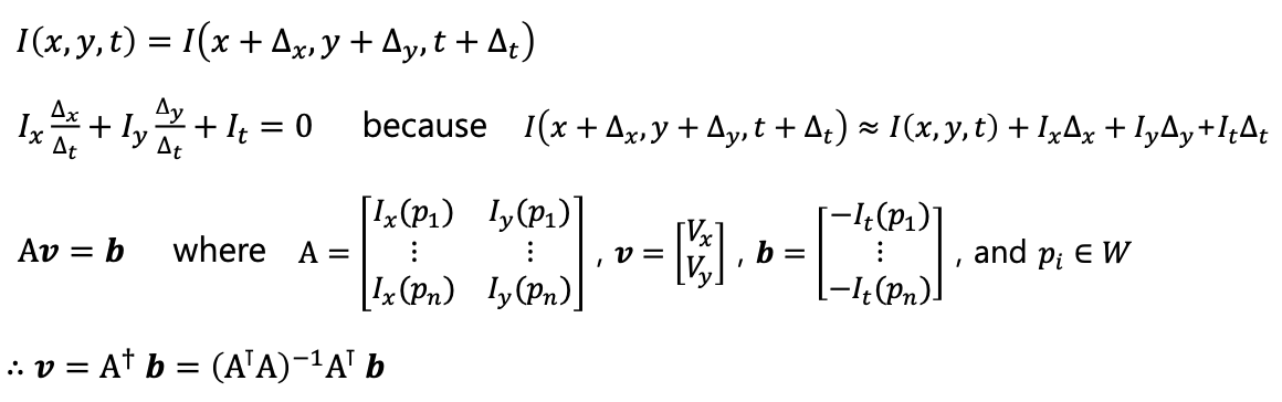
Lukas-Kanade Optical Flow
- Key idea: patch의 움직임을 찾기
-
밝기 불변에 대한 constraint (같은 patch일 경우)
-
- Combination: KLT tracker
- Shi-Tomasi detector (a.k.a. GFTT) + Lukas-Kanade optical flow
cv::goodFeaturesToTrackcv::calcOpticalFlowPyrLK
- Shi-Tomasi detector (a.k.a. GFTT) + Lukas-Kanade optical flow
Solving Non-linear Least Squares with Ceres Solver
- $\underset{\mathbf{m}}{\arg \min } \sum_i \rho_i\left(\left|r_i(\mathbf{m})\right|^2\right)$
- residual function (or cost function or error function) 정의
ceres::Problem을 인스턴스화하고 멤버 함수AddResidualBlock()을 사용하여 residuals를 추가- 각 residual $r_i$를
Ceres::Costfunction형태로 인스턴스화하고 추가- 미분(Jacobian) 계산 방법을 선택
ceres::AutoDiffCostFunctionceres::NumericDiffCostFunctionceres::SizedCostFunction
- cf. 편의성과 성능을 위해서는 chain rule을 사용하는 Automatic derivation 방법이 권장됨
- 미분(Jacobian) 계산 방법을 선택
ceres :: Lossfunction$\rho_i$를 인스턴스화하고 추가 (problem이 outliers에 대한 견고성이 필요한 경우)
- 각 residual $r_i$를
ceres::Solver::Options와ceres::Solver::Summary를 인스턴트화하고 옵션 셋팅- Run
ceres::Solve()
- Solving General Minimization
-
General Minimization ⇒ $\underset{\mathbf{x}}{\arg \min } f(\mathbf{x})$
Non-linear Least Squares General Minimization Ceres::Costfunction ceres::FirstOrderFunction / ceres::GradientFunction ceres::Problem ceres::GradientProblem ceres::Solver ceres::GradientProblemSolver
-
Robust Parameter Estimation
- Bottom-up Approaches (~ Voting)
(e.g. line fitting, relative pose estimation)
Hough transform-
datum은 multiple parameter 후보들에 투표
→ cf. parameter space는 다차원 히스토그램(이산화)으로 유지
- Score: 데이터별 hit 횟수
- Selection: 투표 후 히스토그램에서 peak 찾기
-
RANSAC family- 데이터 샘플들이 single parameter 후보에 투표
- Score: Inlier 후보의 개수 (error는 threshold 사이에 있음)
-
Selection: RANSAC 반복 중에 최고의 모델을 유지
→ cf. RANSAC은 많은 parameter 추정 반복 및 error 계산을 포함함
- Top-down Approaches
(e.g. graph SLAM, multi-view reconstruction)
M-estimator- 모든 데이터는 initial guess로부터 squared errors의 합을 최소로하는 best parameter를 찾는 것을 목표로 함
-
Score: A cost function
→ cost function은 truncated loss function을 포함함
-
Selection: gradient에 따른 cost function이 최소가 될 때
→ cf. Nonlinear optimization는 계산량이 많으며, local minima가 발생할 수 있음